Dennis DeTurck, Herman Gluck, Rafal Komendarczyk, Paul Melvin, David Shea Vela-Vick and I have just put our paper “Triple linking numbers, ambiguous Hopf invariants and integral formulas for three-component links” on the arXiv.

The basic background for the paper is as follows. In 1958 the astrophysicist Lodewijk Woltjer was studying the Crab Nebula when he discovered that there is a certain quantity which is constant for a force-free magnetic field in a closed system (he had argued in an earlier paper that the magnetic fields in the Crab Nebula are force-free). This quantity turns out to be important in, e.g., plasma physics. H. K. Moffatt coined the term “helicity” for this quantity and suggested that it measures the extent to which the field lines wrap and coil around each other.

Vladimir Arnol’d made this more rigorous in his 1973 paper “The asymptotic Hopf invariant and its applications” (which doesn’t appear to be available online) in which he demonstrated that helicity can be thought of as an “average asymptotic linking number”. To explain what that means, I need to digress for a moment into knot theory.

For a mathematician, a knot is just a piece of string where the two ends have been glued together. This can be done in the obvious way or in not so obvious ways. Here’s Wikipedia’s table of all the topologically distinct knots with up to 7 crossings (topologically distinct means you can’t get from one to the other without cutting the string or passing it through itself):

Knot theory is an incredibly rich field in mathematics which is fundamental to the study of three- and four-dimensional spaces and which has applications to everything from shoe-tying to quantum computers.

A collection of two or more knots is called a link. The simplest non-trivial link is the Hopf link:

Here’s a slightly more complicated link (which I drew for this paper):

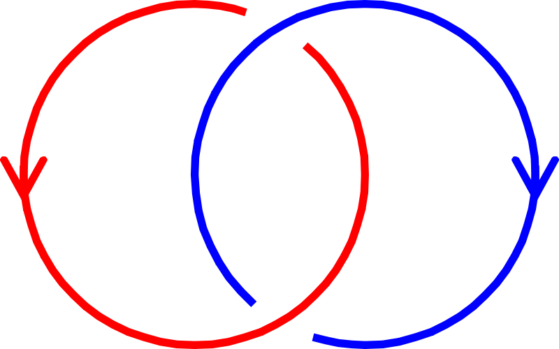
The simplest numerical description of a link is its linking number. I don’t really want to get into the precise definition of the linking number, but it’s easily illustrated by the following three examples. First, a link with linking number zero:

Linking number 1:

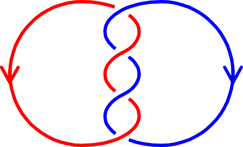
Linking number 2:

Now, getting back to helicity, Arnol’d said that the helicity is an “average asymptotic linking number”. What does the “average asymptotic” business mean? Well, helicity is a property of magnetic fields (or, more generally, of vector fields). Given a magnetic field, you could put two charged particles in the field at different points. Since they’re charged, the two particles will start moving, tracing out two paths (called orbits of the field). If you keep track of the paths for a long time T, you’ll get two long curves in space; close them up and you’ll have two loops in space. Now, a loop in space is just a knot, and two knots form a link, so there’s a linking number between these two loops. If you let T go to infinity and take an appropriate average, you get the average asymptotic linking number of the two orbits, which Arnol’d tells us is equal to the helicity of the field.

This is all very nice, but there’s a slight problem. Helicity is a useful quantity in plasma physics in part because it provides a lower bound for the field energy (this was also proved by Arnol’d). Any magnetic field has an intrinsic energy which has a tendency to decrease as the field evolves toward equilibrium. If the field has non-zero helicity, then you know that the intrinsic energy of the field can’t decrease below a certain amount related to the helicity. This means that, if you know the helicity of a field, then you can determine what that field’s equilibrium energy will be.

The problem is that this doesn’t go both ways: having zero helicity doesn’t necessarily mean that the field can relax to a zero-energy state. So the question, posed by Arnol’d and Boris Khesin in their book Topological Methods in Hydrodynamics, is this: are there “higher-order” helicities which would kick in when the ordinary helicity is zero and provide lower bounds for the field energy?

The problem, then, is to come up with a sensible definition for a higher-order helicity. Recall that Arnol’d showed that the ordinary helicity is an average asymptotic linking number. There is a beautiful integral formula which computes the linking number of two closed curves discovered by Gauss back in 1833, known as the Gauss linking integral (brief aside: see the papers by DeTurck and Gluck and Vela-Vick and me for generalizations of the Gauss linking integral). Using Arnol’d’s approach, it’s fairly straightforward to derive the formula for helicity from the Gauss integral.

That works great for the ordinary helicity, so one might hope something similar will work to get to higher-order helicities. Remember that I said that the linking number is the simplest numerical description (more precisely: topological invariant) of a link, but it’s certainly not the only one. In fact, the linking numbers are useless for one of the simplest three-component links, the Borromean rings:

The salient feature of the Borromean rings is that it’s a non-trivial link (meaning it can’t be pulled apart without breaking one of the components), but deleting any one component causes the whole thing to fall apart. The linking numbers between components are all zero, so you need a more sophisticated measure than the linking number to describe what’s going on.

This measure was provided by John Milnor in his senior thesis(!) in which he classified three-component links up to “link-homotopy”. Milnor came up with a new invariant which I’ll just call μ (though the μ usually comes with various decorations). The definition of μ is actually quite unpleasant, but it is equal to 1 for the Borromean rings and 0 for the trivial three-component link.

Now, by analogy with the Arnol’d approach for ordinary helicity, you might hope that a suitable “average asymptotic μ invariant” would give a higher-order helicity. However, in order to get a useful formula for such a higher-order helicity, you need some sort of integral formula for the μ invariant which is analogous to the Gauss integral. That’s one of the results in our paper (which I’ve finally got back around to mentioning): we give an integral formula for the μ invariant in the cases where that makes sense.

To get there, we related Milnor’s μ invariant to another topological invariant, the Hopf invariant. The basic idea is this: any three-component link is fairly naturally associated to a map from a space called the 3-torus (which naturally lives in 4-dimensional space) to the 2-sphere (think of the surface of the Earth). Such maps were classified (up to homotopy) by Lev Pontryagin in a 1941 paper; the key invariant defined by Pontryagin, denoted by ν, is a generalized (and somewhat ambiguous) version of the usual Hopf invariant and is typically called either the Hopf invariant or the Pontryagin-Hopf invariant.

Our main result is that the μ invariant of a three-component link is equal to half the Pontryagin-Hopf invariant of the associated map. We have two different proofs of this, one purely topological (including the picture at the top of this post) and one more algebraic (following a key insight of Nathan Habegger and Xiao-Song Lin).

Okay, that’s probably not enough detail for the mathematicians and probably way too much for everybody else, so I think I’ll stop here.